Make your own hologram!
Holograms are mystical things, right? Well, actually holograms are just representations of a light field.
Rather confusingly, we sometimes use the word to also represent the recreation of them too.
So you know what you’re getting yourself in for, here’s what we’ll be making today.
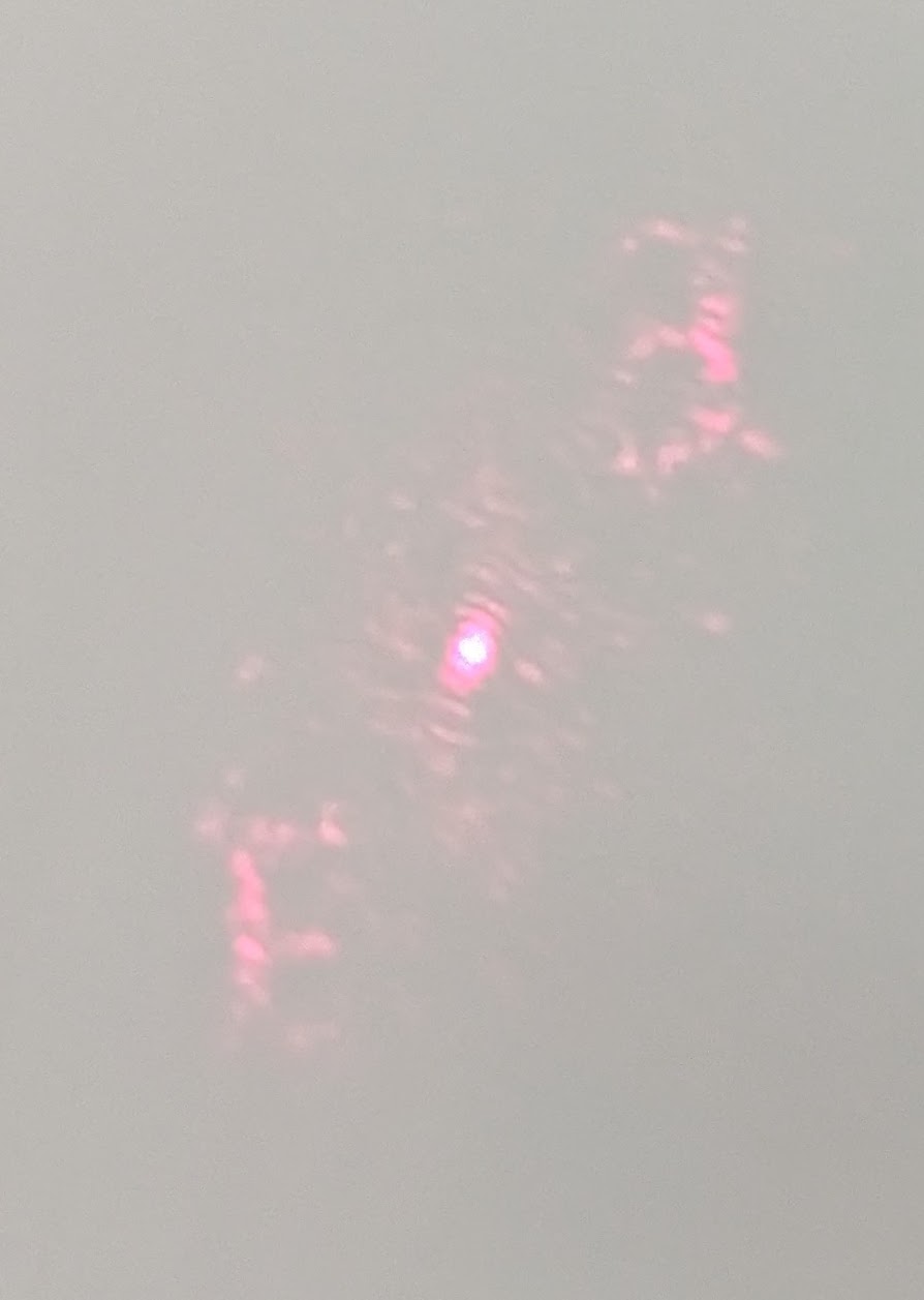
The resultant image from the hologram was generated using the code in the article below.
Yeah, not particularly impressive by itself, but when you look where it comes from, you’ll probably start asking a few questions.
Well, what we’re actually making is a transparency, with certain parts black, and other parts transparent. But when you shine a laser on it (in this case, a red one), after a few metres, it looks like this.
This won’t work for an LED light source, because of its coherence (which means the waves can add and subtract).
Generating the Hologram
As with everything in Python, we start with some imports. Since the code is in Python, you should be able to convert it MATLAB/Julia/your language of choice without much hassle. If you don’t have a working Python install, I recommend using Miniconda.
import numpy as np
import matplotlib.pyplot as plt
from skimage import color, transform
We load in an image, which we binarize (because anything else probably won’t show up nicely).
# Load and binarize the image
path_to_hologram = "/path/to/hologram.png"
img = io.imread(path_to_hologram)
img = transform.resize(img, (128, 128))   # Don't change this, this is important
img = color.rgb2gray( img)  # The hologram only works with one colour at a time
img = img > 0.5 * np.maximum(img)  # Binarize it

plt.figure()
plt.imshow(img, cmap="gray")
plt.title("Original (binarized) Image")
plt.show()
I’ve been at the University of Exeter for a little while now. I thought I’d use (a subset of) the uni’s logo for my hologram target.
If you’ve seen the hologram at the beginning of the page, you might understand where we’re going here, but we’re going to pad our image out to specifically be 300 x 300 pixels.
# Set up parameters
height, width = 300, 300  # Don't change these, these are important

# Pad the image
padded_img = np.zeros((height, width))
padded_img[-img.shape[0]:, :img.shape[1]] = img

plt.figure()
plt.imshow(padded_img, cmap="gray")
plt.title("Padded Image")
plt.show()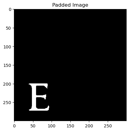
It’s same image as before, but this time with some extra padding.
So now we have the image that we want to display, let’s create a hologram to display it with.
# Initialize our hologram randomly
hologram = np.random.rand(*padded_img.shape) > 0.5

plt.figure()
plt.imshow(hologram, cmap="gray")
plt.title("Initial Hologram")
plt.show()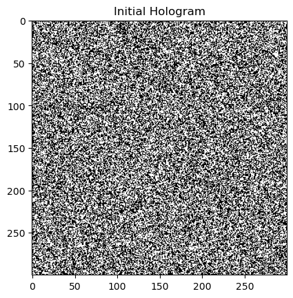
A randomly black and white (300x300) picture, destined to become a hologram.
So now we have our hologram, but this doesn’t give us anything like what we need to have to create our desired imaging target. We have patterned our incoming light, but randomly.
Light travelling in free space (after a long enough distance) performs something called a Fourier transform. If I made more time for this blog, I would talk about it at length.
Basically, the way our algorithm works is to propagate the hologram to far away (we call this, the far field), and then apply the constraint that it must look like the image. Then we propagate that new field back to our hologram and apply the constraint that it must be binary. A more sophisticated approach would have some early stopping, and 50 iterations are probably enough, but CPU cycles are cheap.
def fft2_shifted(x):
    """Compute 2D FFT with frequency shift."""
    return np.fft.fftshift(np.fft.fft2(np.fft.ifftshift(x, axes=(-1, -2)), norm="ortho"), axes=(-1, -2))

def ifft2_shifted(k):
    """Compute 2D IFFT with frequency shift."""
    return np.fft.fftshift(np.fft.ifft2(np.fft.ifftshift(k, axes=(-1, -2)), norm="ortho"), axes=(-1, -2))

# Iterative Fourier Transform Algorithm (IFTA)
for _ in range(1000):
    # Propagate to Fourier plane using FFT
    fft_hologram = fft2_shifted(hologram)

    # Apply target intensity constraint at the Fourier plane
    fft_hologram = np.sqrt(padded_img) * np.exp(1j * np.angle(fft_hologram))

    # Propagate back to the object plane using IFFT
    hologram = ifft2_shifted(fft_hologram)

    # Apply binary amplitude constraint at the object plane
    hologram = hologram > 0

# Display the binary amplitude hologram
plt.figure()
plt.imshow(hologram, cmap="gray")
plt.title("Final Hologram")
plt.show()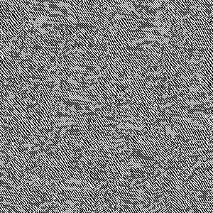
A freshly made hologram, it doesn’t look like much right now, but just think about what happens with a laser on it.
Now, this is all well and good, but what’s the result of this?
# Save the hologram
io.imsave("final_hologram.png", hologram)

# Display Fourier Transform of the hologram
fft_H = fft2_shifted(hologram - hologram.mean())
plt.figure()
plt.imshow(np.abs(fft_H)**2, cmap="gray")
plt.title("Fourier Transform of Hologram")
plt.show()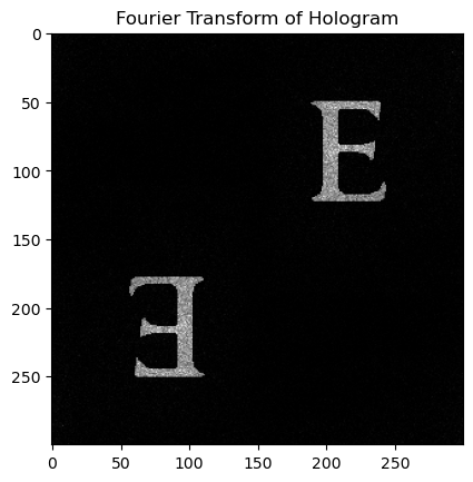
Hey presto. Now we’re playing with portals. You can see that it looks exactly like our target image!
Printing our Hologram
Thankfully this part is much easier than programming anything. First, you need to get some transparent paper that works with your printer. I used this one from amazon.
Just make sure your printer is set to print 600 dpi, and make your image 0.5 in × 0.5 in. This is the reason that our earlier image was 300 × 300, so that one pixel on your image is exactly one dot on your transparency. If your hologram doesn’t work this is probably why.
Using our Hologram
Now simply take your transparency and shine a laser through it. You should see something like we had before. It’s a bit fiddly to hold it up, but if so, find a friend to help.
If you make one at home show me! I’d love to see what you get up to.